IPA polynomial commitment by hand

2023-04-06

This post was originally written on July 2022 during the ‘0xPARC Halo2 learning group’, posting it now as it was forgotten in a hackmd.

Context

During this past month (June 13 - July 8, 2022) I’ve been attending at the Halo2 Learning Group that 0xPARC organized. It has been an amazing experience and I’ve learned a lot from aweseome people. For the past two weeks, the participants were encouraged to do a project related to the contents of the sessions, after a bit of doubts, I’ve chosen to do it about the Inner Product Argument used in Halo2 for the polynomial commitments, which is described in the Halo paper.

I’ve used this opportunity to study how IPA works, reading it from the Halo paper but also from the Bulletproofs paper and the good explanations from the Dalek documentation and the Dankrad Feist article.

Thanks to Ye Zhang, Ying Tong and Haichen Shen for their advise on the papers and resources to study. Also thanks to David Nevado for the typos found in this post.

Intro

This article overviews the IPA construction described in the Halo paper, by doing a step-by-step example with small numbers, following the style done in the “PLONK by Hand series” by Joshua Fitzgerald. This post does not cover the amortization technique proposed in the Halo paper.

Together with this by-hand step-by-step example, I’ve implemented it in Sage and also in Rust using arkworks:

Also, if you’re looking for other Sage/Python IPA implementations, you can find one in the Darkfi/research repo and another one in the Ethereum/research repo.

This post is divided in 3 parts:

IPA overview
IPA by hand
IPA Sage implementation

IPA overview

This section provides an overview on the IPA scheme, for more details it is recommended to go directly to the earlier mentioned papers and articles.

The scheme objective is to allow the prover to prove that the polynomial $p(X)$ from the commitment $P$, evaluates to $v$ at $x$, and that $deg(p(X)) \leq d-1$.

Notation:

Scalar mul: $[a]G$, where $a$ is a scalar and $G \in \mathbb{G}$
Inner product: $<\overrightarrow{a}, \overrightarrow{b}> = a_0 b_0 + a_1 b_1 + \ldots + a_{n-1} b_{n-1}$
Multiscalar mul: $<\overrightarrow{a}, \overrightarrow{G}> = [a_0] G_0 + [a_1] G_1 + \ldots + [a_{n-1}] G_{n-1}$

We have a transparent setup consisting of a random vector of points $\overrightarrow{G} \in^r \mathbb{G}^d$, and a point $H \in^r \mathbb{G}$.

The prover commits to the polynomial $p(X) = \sum^{d-1}_0 a_i x^i$ by a Pedersen vector commitment

\[P=<\overrightarrow{a}, \overrightarrow{G}> + [r]H\]

where $\overrightarrow{a}$ is the vector of the coefficients of $p(X)$. And sets $v$ such that

\[v=<\overrightarrow{a}, \overrightarrow{b} > = <\overrightarrow{a}, \{1, x, x^2, \ldots, x^{d-1} \} >\]

We can see that computing $v$ is the equivalent to evaluating $p(X)$ at $x$ ($p(x)=v$).

Both parties know $P$, point $x$ and claimed evaluation $v$. For $U \in^r \mathbb{G}$.

Now, for $k$ rounds ($d=2^k$, from $j=k$ to $j=1$):

Prover sets random blinding factors: $l_j, r_j \in \mathbb{F}_p$
Prover computes

\[L_j = < \overrightarrow{a}_{lo}, \overrightarrow{G}_{hi}> + [l_j] H + [< \overrightarrow{a}_{lo}, \overrightarrow{b}_{hi}>] U\\ R_j = < \overrightarrow{a}_{hi}, \overrightarrow{G}_{lo}> + [r_j] H + [< \overrightarrow{a}_{hi}, \overrightarrow{b}_{lo}>] U\]
Verifier sends random challenge $u_j$
Prover computes the halved vectors for next round:

\[\overrightarrow{a} \leftarrow \overrightarrow{a}_{hi} \cdot u_j^{-1} + \overrightarrow{a}_{lo} \cdot u_j\\ \overrightarrow{b} \leftarrow \overrightarrow{b}_{lo} \cdot u_j^{-1} + \overrightarrow{b}_{hi} \cdot u_j\\ \overrightarrow{G} \leftarrow \overrightarrow{G}_{lo} \cdot u_j^{-1} + \overrightarrow{G}_{hi} \cdot u_j\]

After final round, $\overrightarrow{a}, \overrightarrow{b}, \overrightarrow{G}$ are each of length 1.

Verifier can compute $G = \overrightarrow{G}_0 = < \overrightarrow{s}, \overrightarrow{G} >$, and $b = \overrightarrow{b}_0 = < \overrightarrow{s}, \overrightarrow{b} >$, where $\overrightarrow{s}$ is the binary counting structure:

\[ s = (u_1^{-1} ~ u_2^{-1} \cdots ~u_k^{-1},\\ ~~~~~~~~~u_1 ~~~ u_2^{-1} ~\cdots ~u_k^{-1},\\ ~~~~~~~~~u_1^{-1} ~~ u_2 ~~\cdots ~u_k^{-1},\\ ~~~~~~~~~~~~~~~~~\vdots\\ ~~~~~~~~~u_1 ~~~~ u_2 ~~\cdots ~u_k) \]

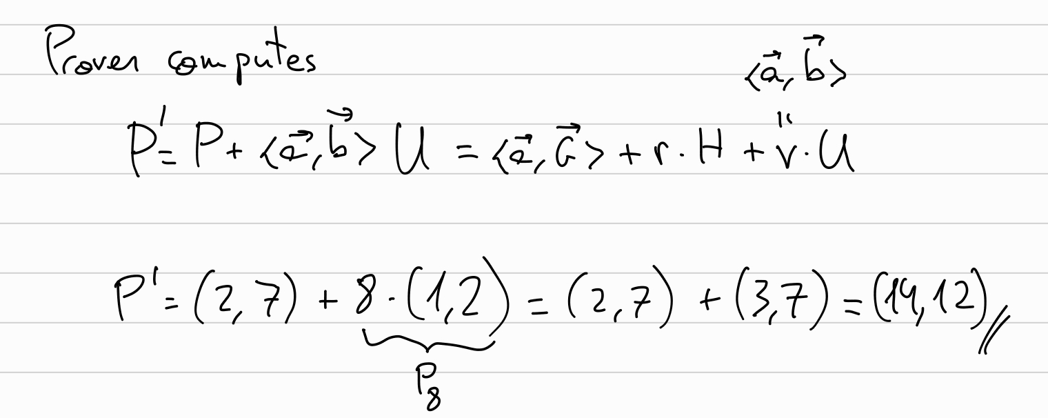
Also, the verifier can computes $P'$ as

\[P' = P + [v] U\]

which under the hood is equivalent to $P'= <\overrightarrow{a}, G> + [r]H + [v] U$.

Then, Verifier checks:

\[[a]G + [r'] H + [ab] U == P' + \sum_{j=1}^k ( [u_j^2] L_j + [u_j^{-2}] R_j)\]

where the $r' = r + \sum_{j=1}^k (l_j u_j^2 + r_j u_j^{-2})$.

We can see how this match if we unfold it (added colors to provide a bit of intuition on the relation of values):

\[ \textcolor{brown}{[a]G} + \textcolor{cyan}{[r'] H} + \textcolor{magenta}{[ab] U} == \textcolor{blue}{P'} + \sum_{j=1}^k ( \textcolor{violet}{[u_j^2] L_j} + \textcolor{orange}{[u_j^{-2}] R_j}) \]

\[ LHS = \textcolor{brown}{[a]G} + \textcolor{cyan}{[r'] H} + \textcolor{magenta}{[ab] U}\\ = \textcolor{brown}{< \overrightarrow{a}, \overrightarrow{G} >}\\ + \textcolor{cyan}{[r + \sum_{j=1}^k (l_j \cdot u_j^2 + r_j u_j^{-2})] \cdot H}\\ + \textcolor{magenta}{< \overrightarrow{a}, \overrightarrow{b} > U} \]

\[ RHS = \textcolor{blue}{P'} + \sum_{j=1}^k ( \textcolor{violet}{[u_j^2] L_j} + \textcolor{orange}{[u_j^{-2}] R_j})\\ = \textcolor{blue}{< \overrightarrow{a}, \overrightarrow{G}>}\\ + \textcolor{blue}{[r] H}\\ + \sum_{j=1}^k ( \textcolor{violet}{[u_j^2] \cdot <\overrightarrow{a}_{lo}, \overrightarrow{G}_{hi}> + [l_j] H + [<\overrightarrow{a}_{lo}, \overrightarrow{b}_{hi}>] U}\\ \textcolor{orange}{+ [u_j^{-2}] \cdot <\overrightarrow{a}_{hi}, \overrightarrow{G}_{lo}> + [r_j] H + [<\overrightarrow{a}_{hi}, \overrightarrow{b}_{lo}>] U})\\ + \textcolor{blue}{[< \overrightarrow{a}, \overrightarrow{b} >] U}\\ \]

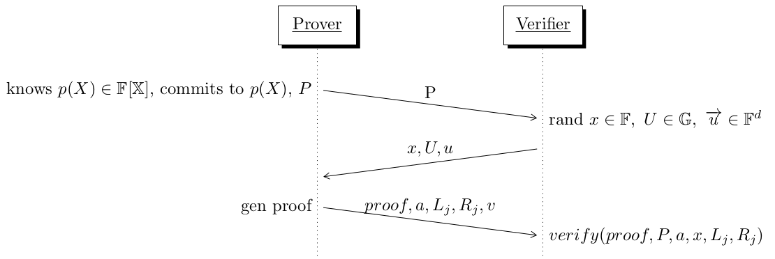
In the following diagram we can see a high level overview of the steps in the protocol:

IPA by hand

This section provides a step-by-step example of IPA with small values, following the style done in the “PLONK by Hand series” by Joshua Fitzgerald.

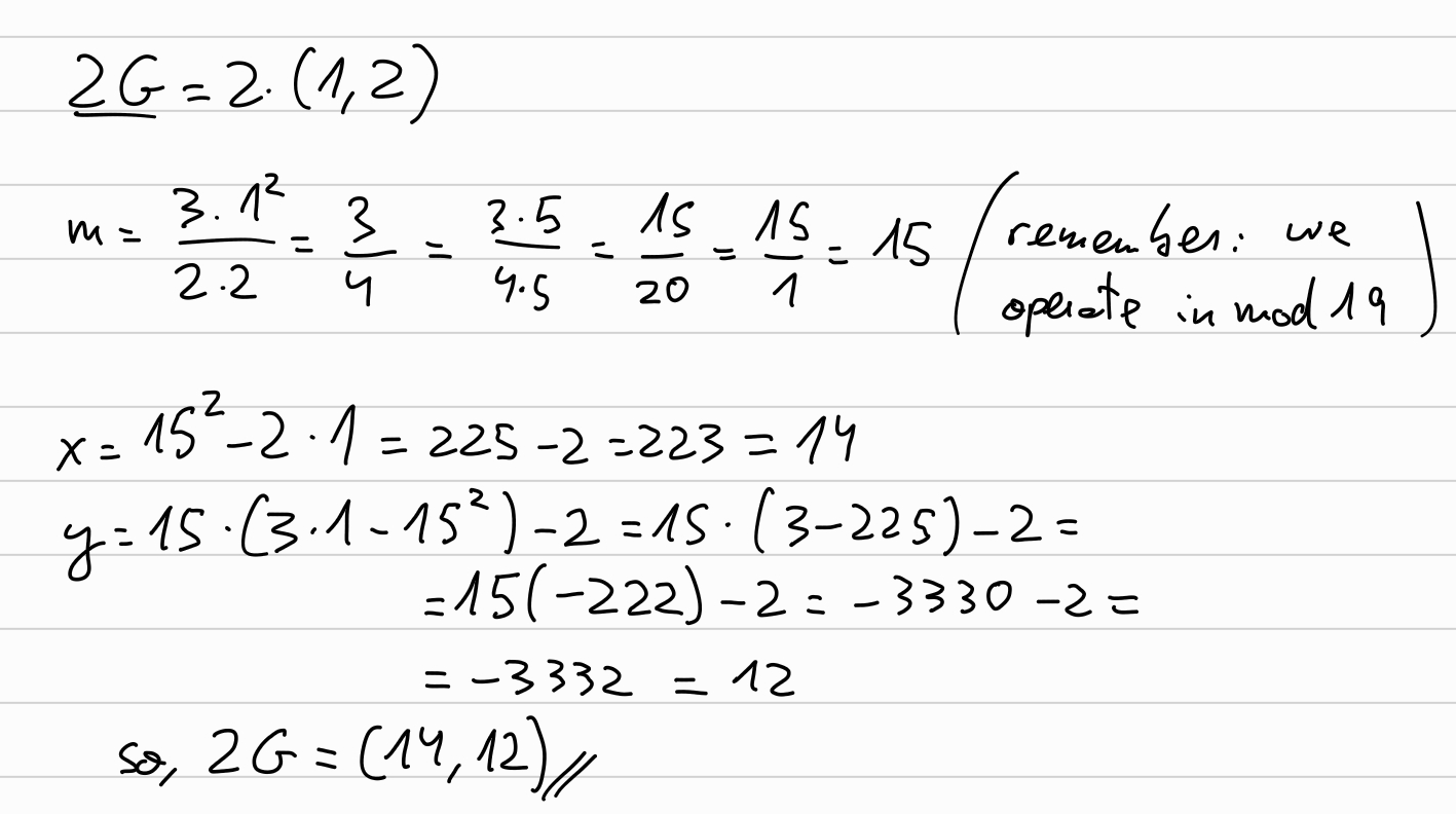
We will use the Elliptic curve $E(\mathbb{F}_{19}): y^2 = x^3 + 3$.

In the same way that was done in the Plonk by hand series, let’s compute all the points from our generator $G=(1,2) \in E(\mathbb{F}_{19})$. We’ll start with $2G$:

Combining point doubling and inverses for $4G, 6G, 8G, \ldots$, together with point addition we obtain all the points of our curve:

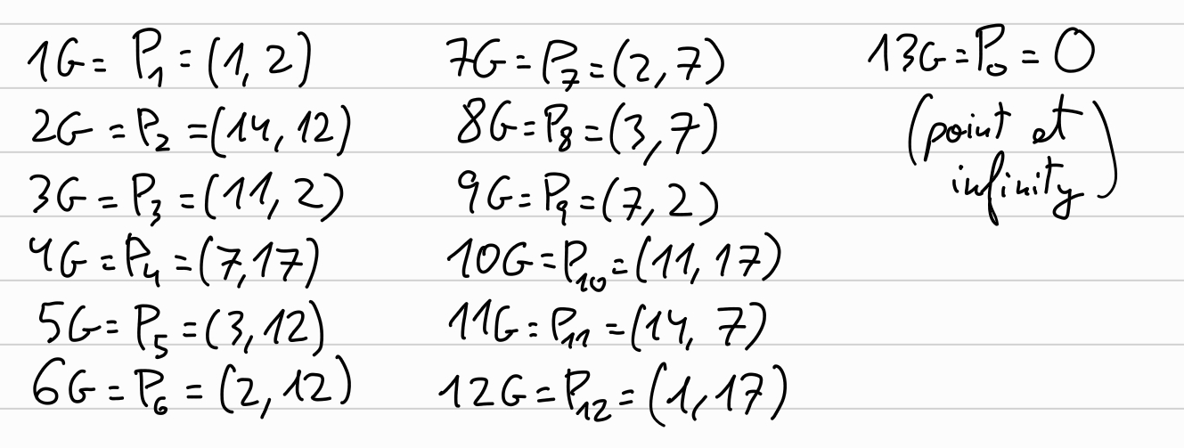
As we find out, $14 G = G$, thus $ord(G)_{E(\mathbb{F}_{19})} = 13$, so we will work in $\mathbb{F}_{13}$.

Before we start the interaction of the protocol, we need to setup some values. First of all, we need to define the degree of the polynomial with which we want to work, we will use the degree $d=8$ to make manual computations shorter.

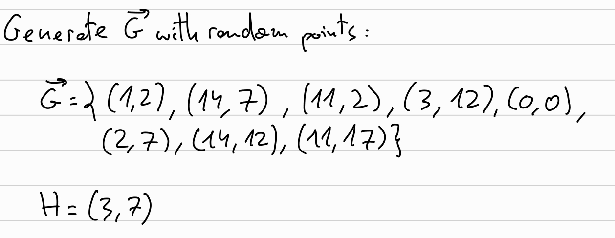
We set up the vector $\overrightarrow{G}$ with random points (without known DLOG between them), and also a random point $H$:

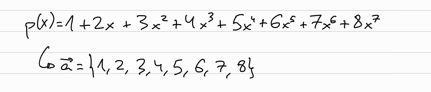
We define our polynomial $p(X)$, to which we want to commit, and let $\overrightarrow{a}$ be its coefficients:

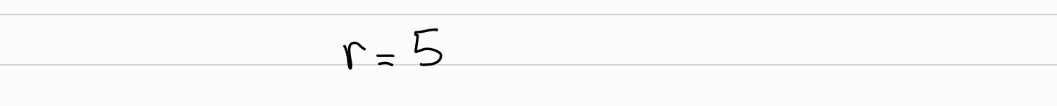
Verifier chooses a random challenge $r$:

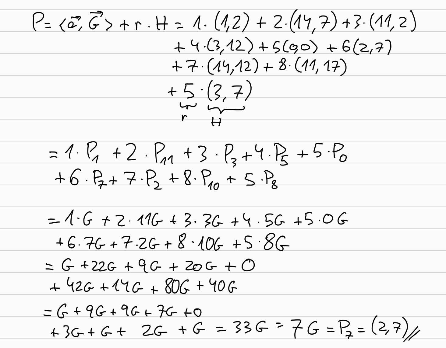
Prover commits to $\overrightarrow{a}$:

We are following the Halo paper, which describes an IPA variant in which the second vector $\overrightarrow{b}$ is fixed for the given choice of $x$, being $\overrightarrow{b} = {1, x, x^2, x^3, \ldots, x^{d-1}}$.

We will use $x=3$, being $\overrightarrow{b}$:

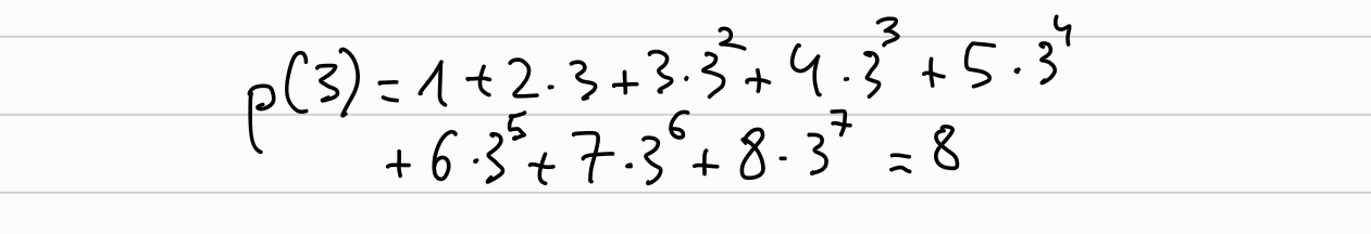
Now the prover computes the inner product between $\overrightarrow{a}$ and $\overrightarrow{b}$, using

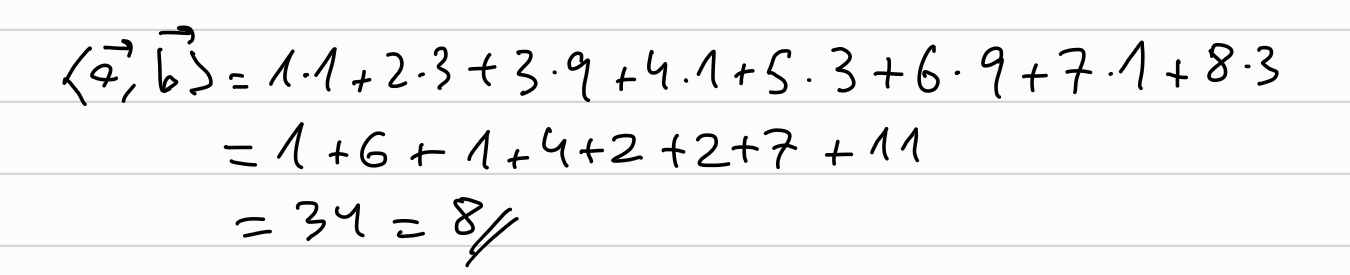
Which, since our choose of $\overrightarrow{b}$, it is the equivalent than evaluating $p(X)$ at $x=3$:

Now the verifier generates the random challenges $u_j \in \mathbb{I}$ and $U \in E$:

In a non-interactive version of the protocol, these values would be obtained by hashing the transcript (Fiat-Shamir).

The prover computes P’ Followed by $k=log(d)$ (3) rounds explained below.

Rounds

For each round, from $k-1$ to $0$, prover will compute:

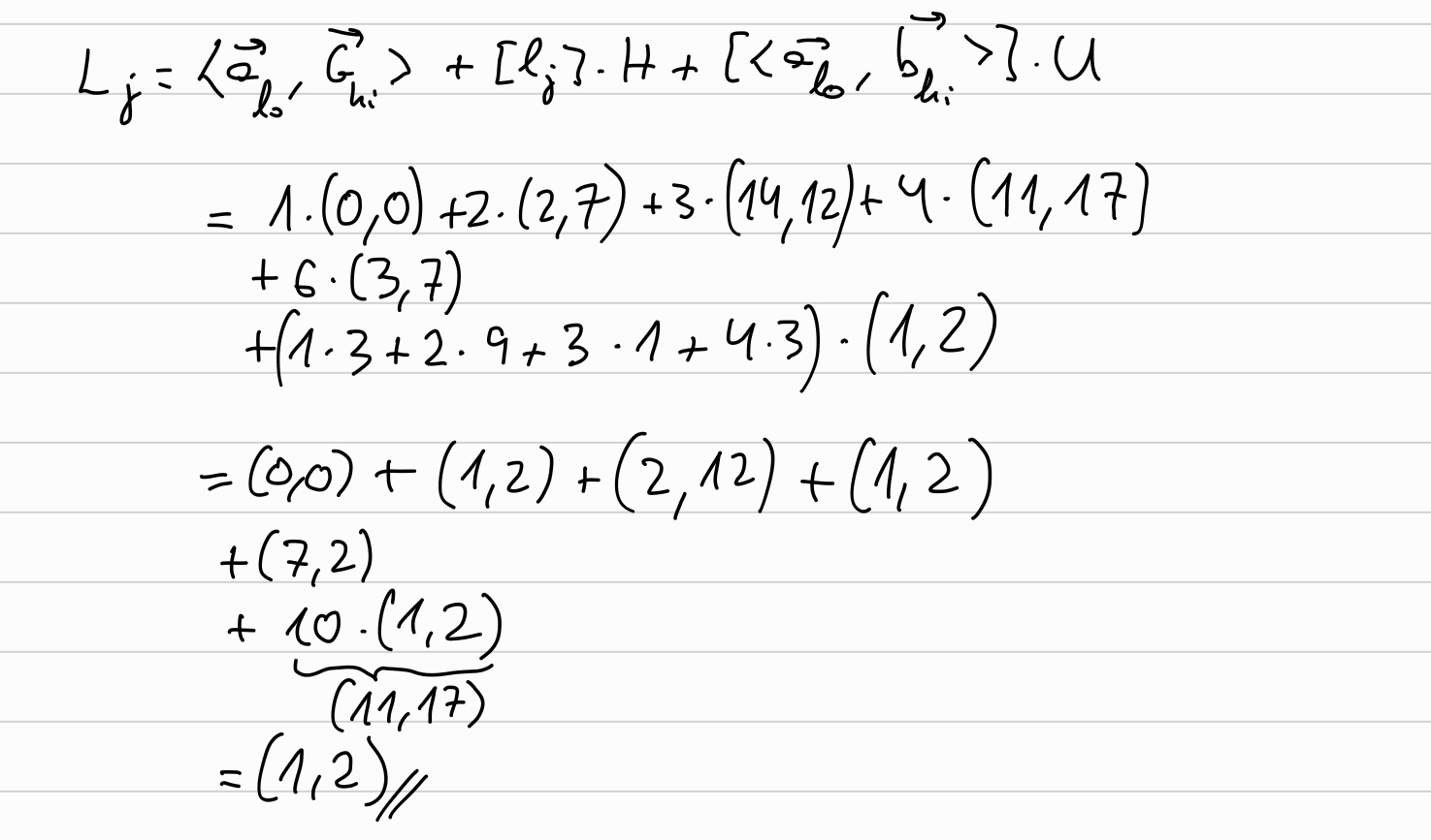
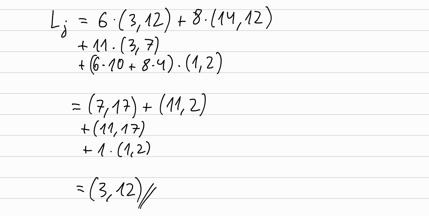
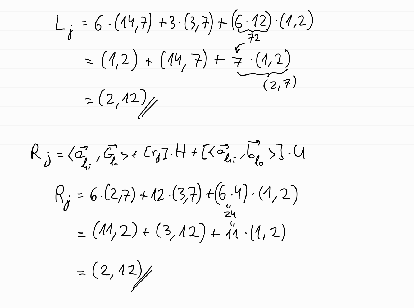
\[ L_j = \langle \overrightarrow{a}_{lo}, \overrightarrow{G}_{hi} \rangle + [l_j] H + [\langle \overrightarrow{a}_{lo}, \overrightarrow{b}_{hi} \rangle] U \]

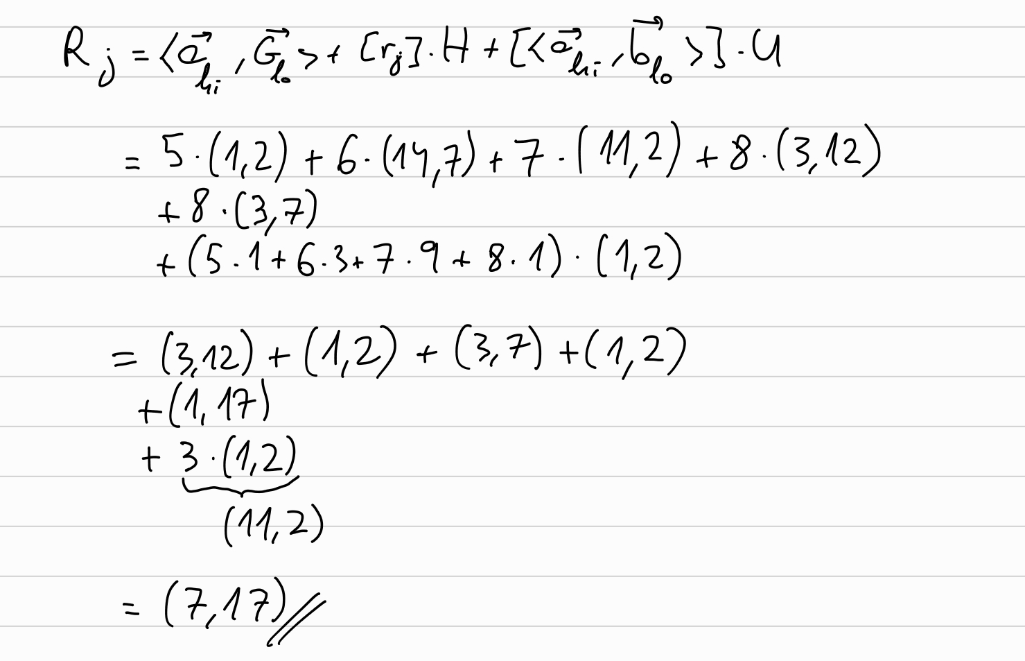
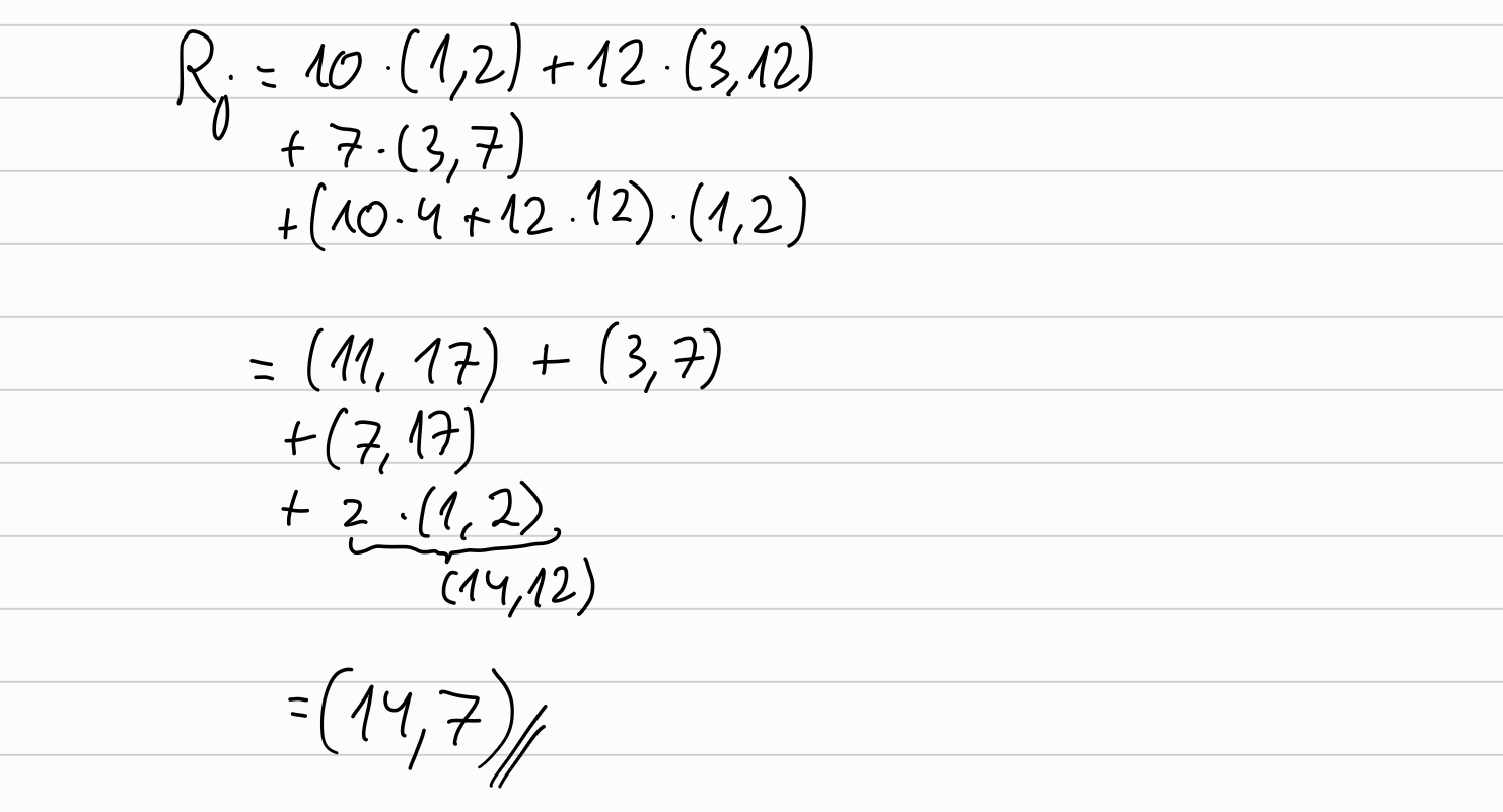
\[ R_j = \langle \overrightarrow{a}_{hi}, \overrightarrow{G}_{lo} \rangle + [r_j] H + [\langle \overrightarrow{a}_{hi}, \overrightarrow{b}_{lo} \rangle] U \]

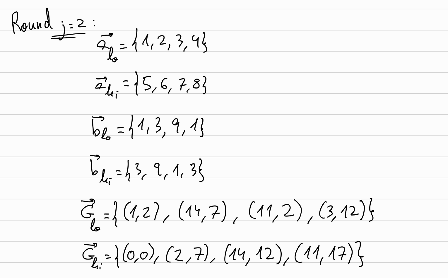
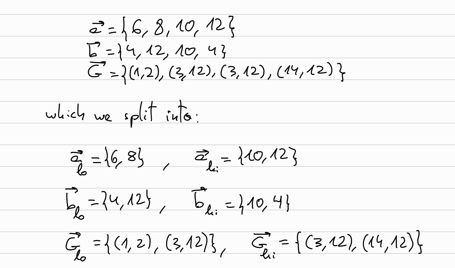
Round j=2:

So, first we will split $\overrightarrow{a}, \overrightarrow{b}, \overrightarrow{G}$ into their respective left and right halves ($\overrightarrow{v}_{lo}, \overrightarrow{v}_{hi}$):

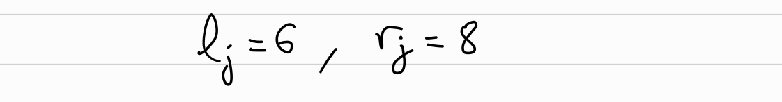
Set random blinding factors $l_2, r_2$:

And let’s calculate $L_2$:

And the same with $R_2$:

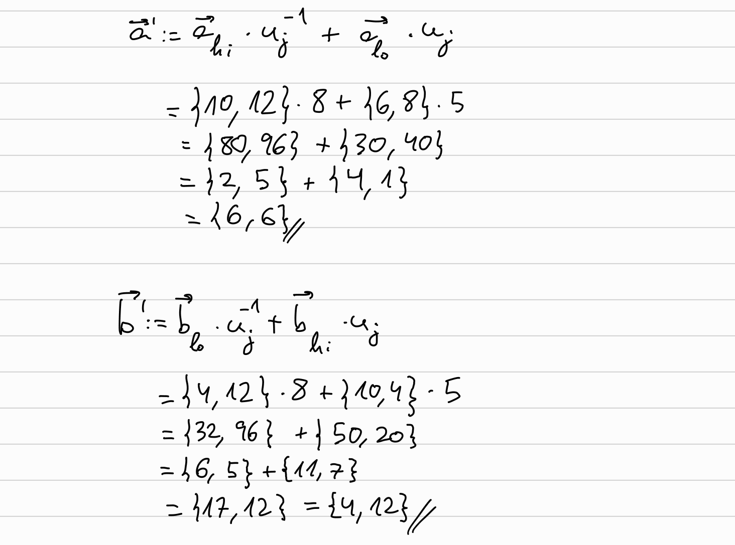
Now, we will compute the new $\overrightarrow{a}, \overrightarrow{b}, \overrightarrow{G}$ to be used in the next round by:

\[ \overrightarrow{a} \longleftarrow \overrightarrow{a}_{hi} \cdot u_j^{-1} + \overrightarrow{a}_{lo} \cdot u_j\\ \overrightarrow{b} \longleftarrow \overrightarrow{b}_{lo} \cdot u_j^{-1} + \overrightarrow{b}_{hi} \cdot u_j \]

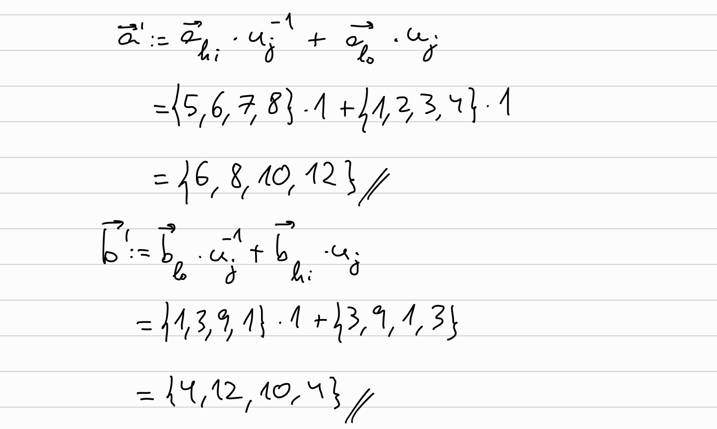
And similarly for $\overrightarrow{G} \longleftarrow \overrightarrow{G}_{lo} \cdot u_j^{-1} + \overrightarrow{G}_{hi} \cdot u_j$

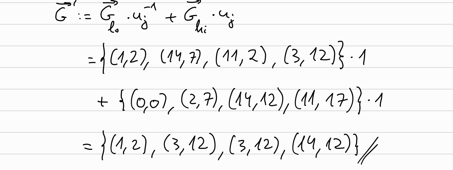
We can see that $\overrightarrow{a}, \overrightarrow{b}, \overrightarrow{G}$ have halved.

Round j=1:

From the previous round we have:

Choose the random blinding factors:

And now, in the same fashion that we did in the previous round, we compute the $L_1, R_1$:

Now, we will compute the new $\overrightarrow{a}, \overrightarrow{b}, \overrightarrow{G}$ to be used in the next round:

Round j=0:

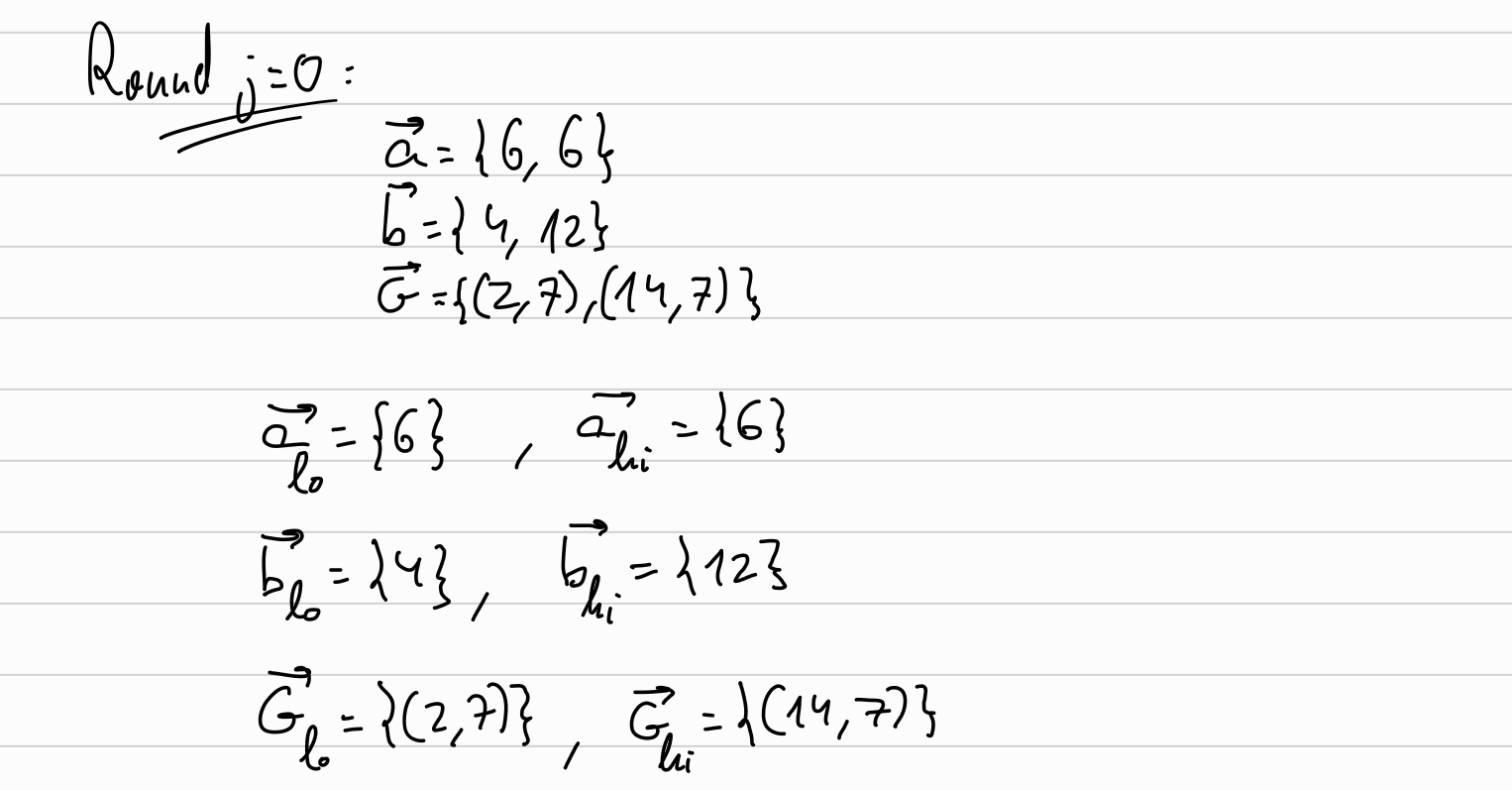
Set the random blinding factors $l_0, r_0$:

Compute $L_0, R_0$:

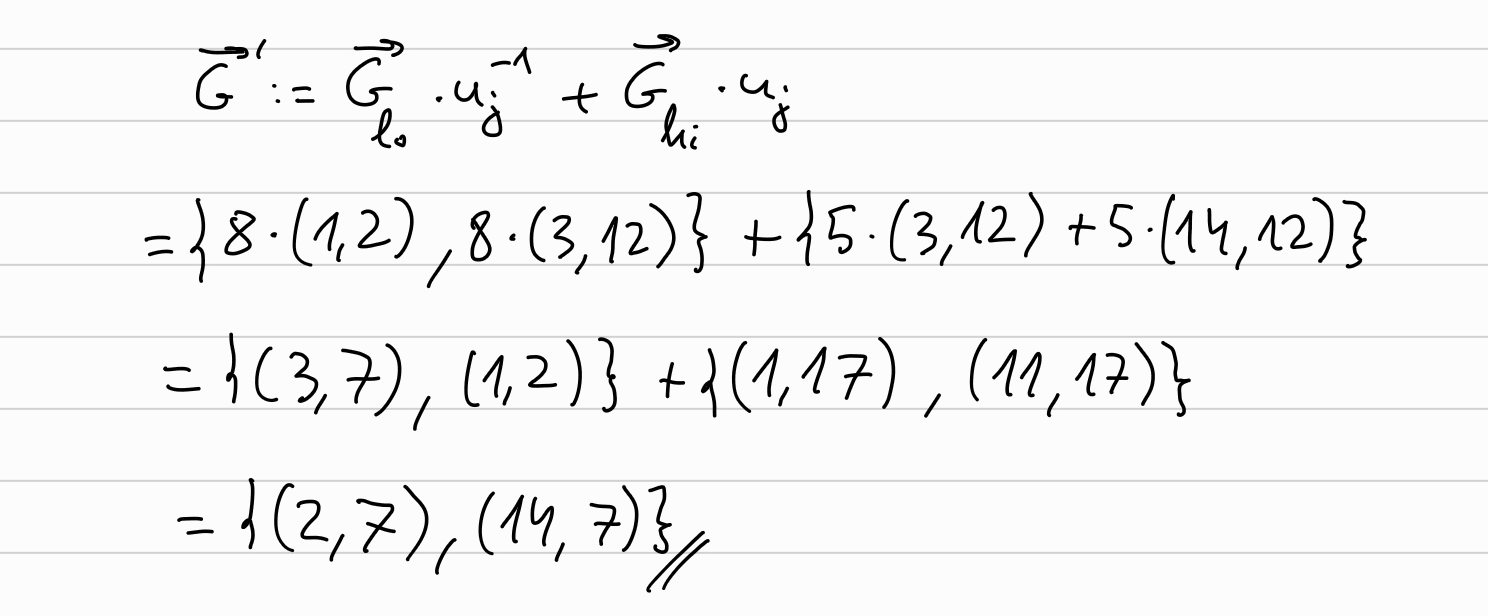
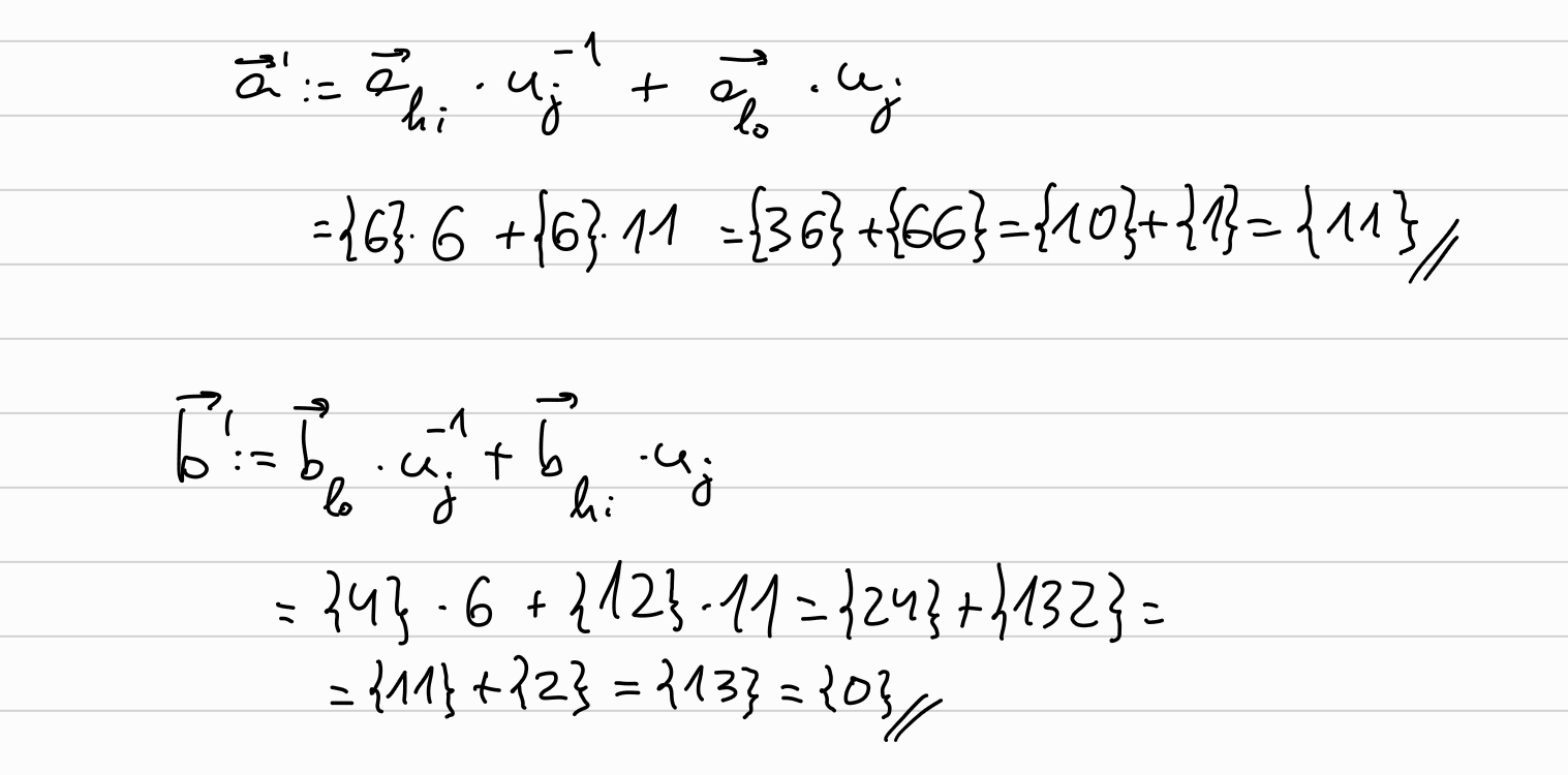
we will compute the new halved $\overrightarrow{a}, \overrightarrow{b}, \overrightarrow{G}$:

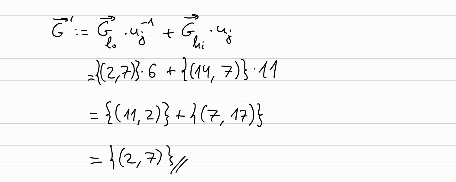
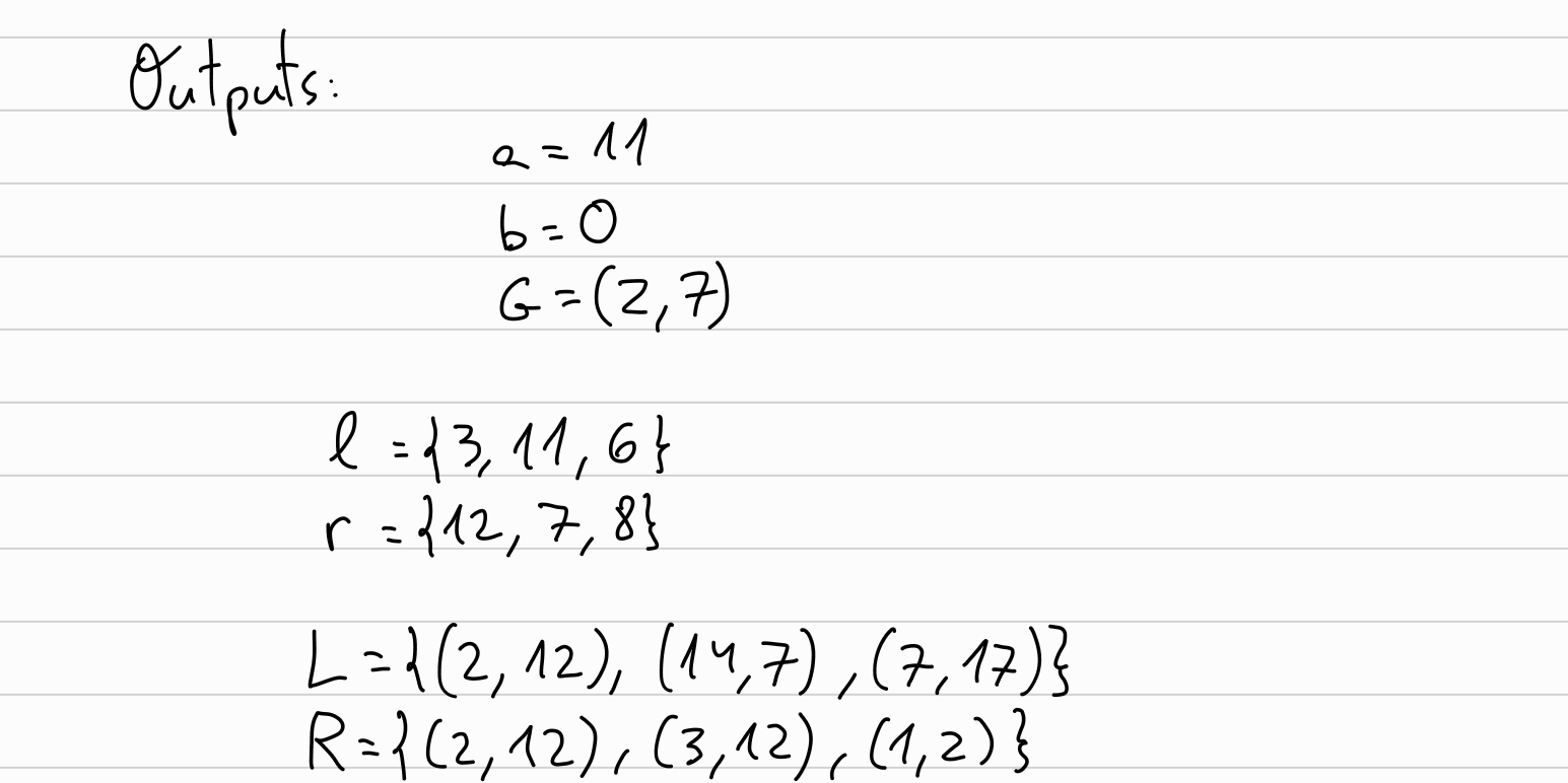
The prover ends having as outputs $a=\overrightarrow{a}_0, ~~b=\overrightarrow{b}_0, ~~G=\overrightarrow{G}_0$, and the random blinding factors $\overrightarrow{l}, \overrightarrow{r}$, together with $\overrightarrow{L}, \overrightarrow{R}$:

Verify

First, verifier recomputes $b$ and $G$. This can be done in more efficient ways described in the Halo paper, but for the sake of simplicity we will assume that the verifier computes $b$ and $G$ in the naive way (which is, doing a similar loop than what the prover did, going from the original $\overrightarrow{b}, \overrightarrow{G}$ halving each round until obtaining $b, G$). In the Sage implementation provided in the next section, we will use the efficient approach, which was also provided in the overview section.

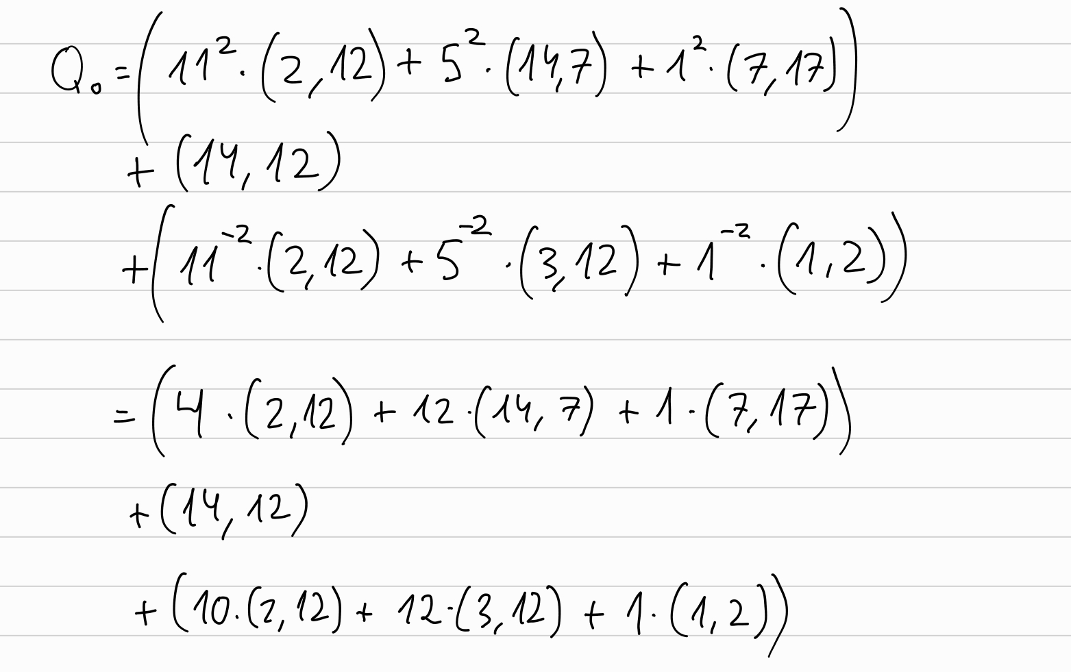
Now, the verifier can compute $P'$ in the same way that the prover did ($P'=P + [v] U$), and from here computes $Q_0 = \sum_{j=1}^k ( [u_j^2] L_j) + P' + \sum_{j=1}^k ([u_j^{-2}] R_j)$:

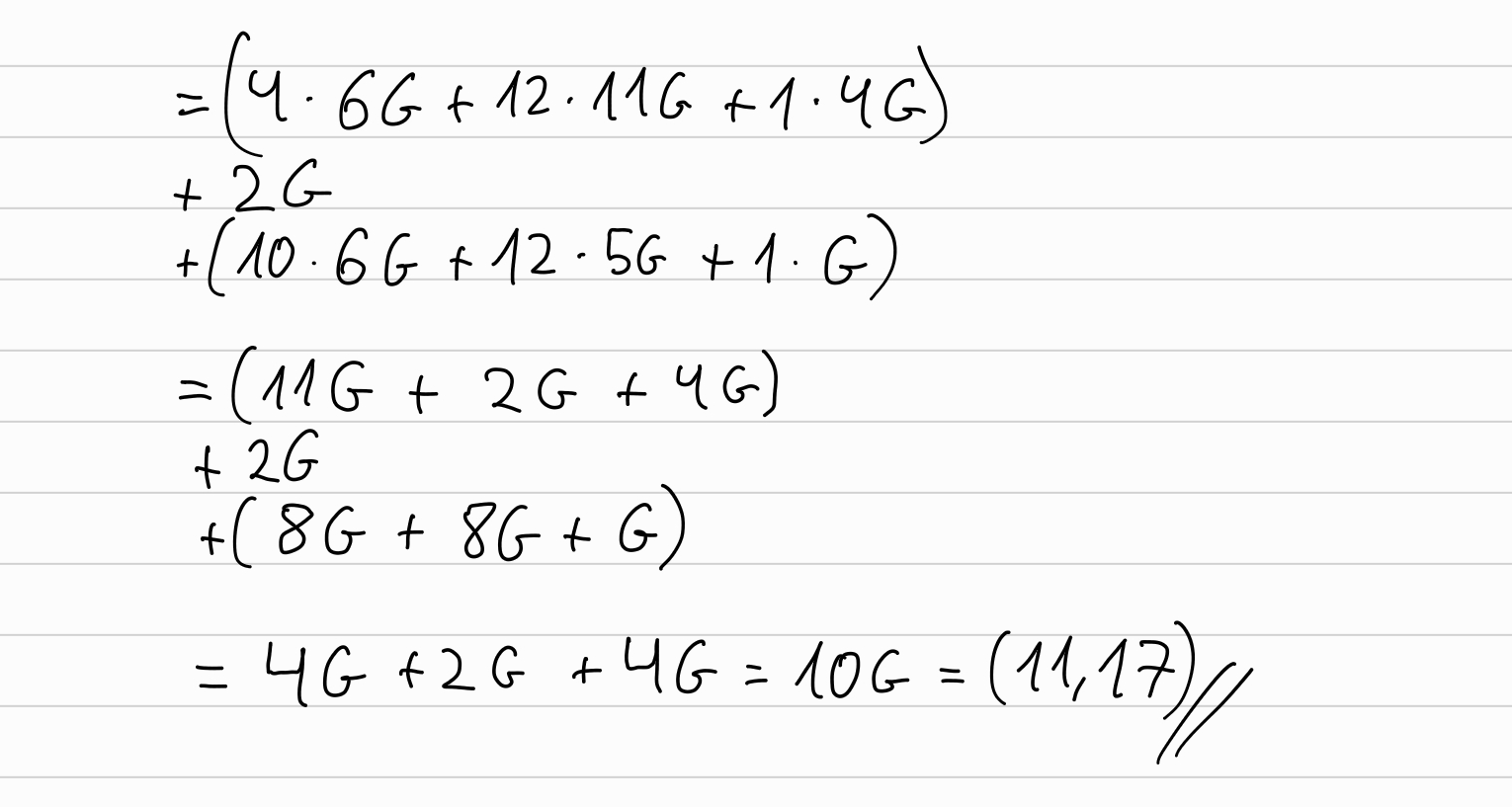
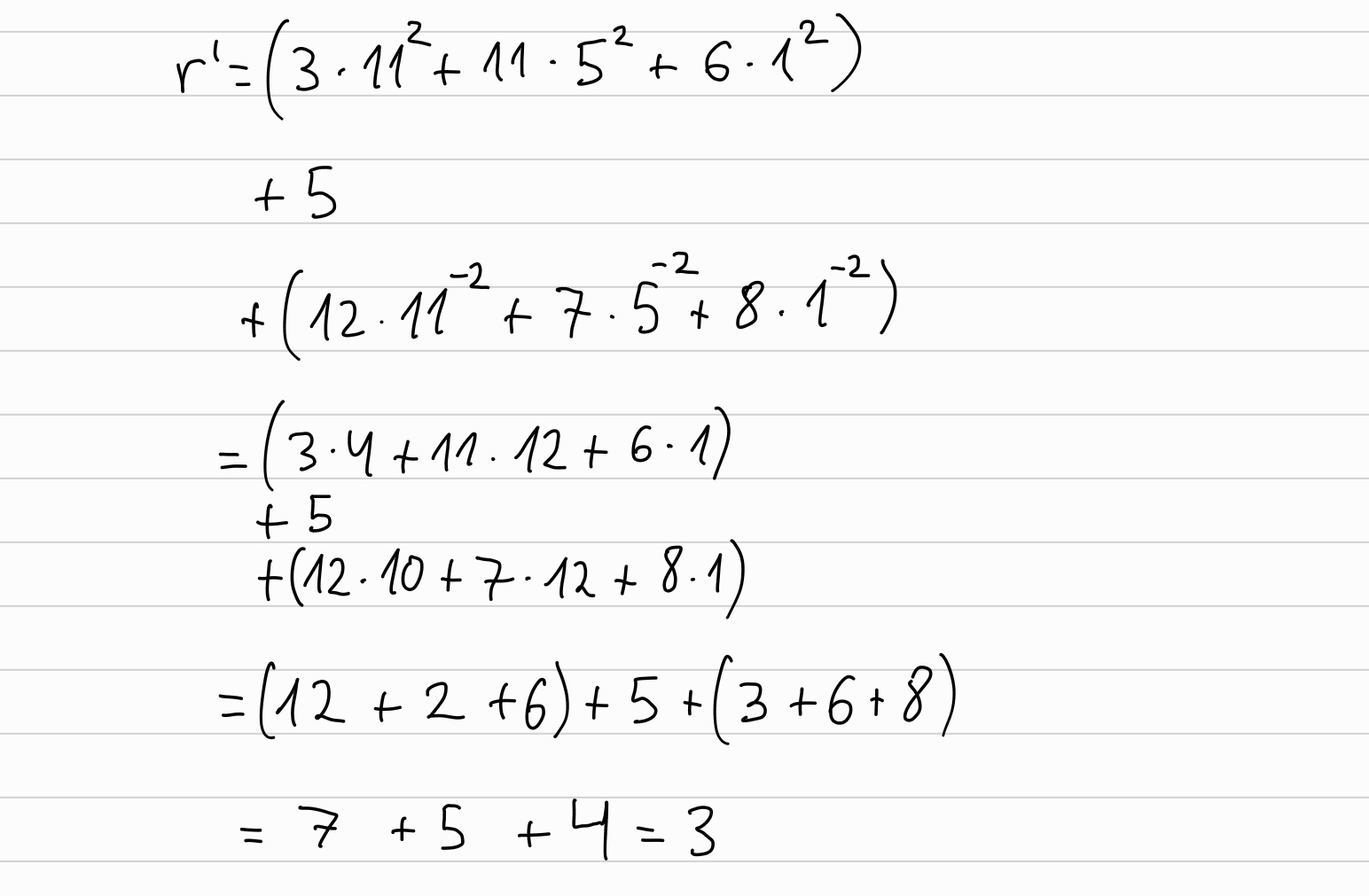
As we did previously, for an easier by-hand computation, we can ‘translate’ the points to multiples of the generator $G$, to operate with them more easily without a computer:

We need to compute also $r' = \sum_{j=1}^k (l_j \cdot u_j^2) + r + \sum_{j=1}^k (r_j \cdot u_j^{-2})$:

And then compute $Q_1 = [a] G + [r'] H + [ab] U$:

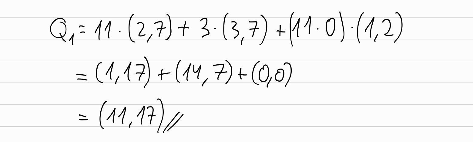
And by checking that $Q_0 == Q_1$, the verifier finishes the verification.

Now let’s do a simple implementation

We will do a simple implementation in Sage of the protocol.

First of all, we set up our curve:

p = 19
Fp = GF(p)
E = EllipticCurve(Fp,[0,3])
g = E(1, 2)
q = g.order()
Fq = GF(q)

Now let’s create the ‘IPA’ class:

class IPA_halo(object):
    def __init__(self, F, E, g, d):
        self.g = g
        self.F = F
        self.E = E
        self.d = d

        self.h = E.random_element()
        self.gs = random_values(E, d)
        self.hs = random_values(E, d)


def random_values(G, d):
    r = [None] * d
    for i in range(d):
        r[i] = G.random_element()
    return r

Now we can generate all the elliptic curve points in a similar way that when we computed them by-hand in the previous section:

print("\nlet's generate all the points:")
P = g+g
print("P_0:", g)
i=1
while P!=g:
    print("P_%d:" % i, P)
    P = P + P
    i += 1
print("P_%d:" % (i+1), E(0), "(point at infinity)")

Alternatively we can use Sage’s methods:

# alternatively:
print("points", E.points())
print("number of points", len(E.points()))

Now, the Prover will set the polynomial $p(X)$ and the Verifier would set $x$:

print("\ndefine p(X) = 1 + 2x + 3x² + 4x³ + 5x⁴ + 6x⁵ + 7x⁶ + 8x⁷")
a = [ipa.F(1), ipa.F(2), ipa.F(3), ipa.F(4),
    ipa.F(5), ipa.F(6), ipa.F(7), ipa.F(8)]
x = ipa.F(3)
x_powers = powers_of(x, ipa.d) # = b

Prover sets the blinding factor $r$:

r = int(ipa.F.random_element())

We will implement some utility functions that we’ll use later in the rest of the implementation:

def inner_product_field(a, b):
    assert len(a) == len(b)
    c = 0
    for i in range(len(a)):
        c = c + a[i] * b[i]

    return c

def inner_product_point(a, b):
    assert len(a) == len(b)
    c = 0
    for i in range(len(a)):
        c = c + int(a[i]) * b[i]

    return c

def vec_add(a, b):
    assert len(a) == len(b)
    return [x + y for x, y in zip(a, b)]

def vec_mul(a, b):
    assert len(a) == len(b)
    return [x * y for x, y in zip(a, b)]

def vec_scalar_mul_field(a, n):
    r = [None]*len(a)
    for i in range(len(a)):
        r[i] = a[i]*n
    return r

def vec_scalar_mul_point(a, n):
    r = [None]*len(a)
    for i in range(len(a)):
        r[i] = a[i]*int(n)
    return r

And we will implement in the IPA class the methods for committing and evaluating:

class IPA_halo:
    # [...]
    def commit(self, a, r):
        P = inner_product_point(a, self.gs) + r * self.h
        return P

    def evaluate(self, a, x_powers):
        return inner_product_field(a, x_powers)

So now the prover can commit to $a$:

print("\nProver commits to a:")
P = ipa.commit(a, r)
print(" commit: P = <a, G> + r * H = ", P)
print("Evaluates a at {1 + x + x² + x³ + … + xⁿ⁻¹}:")
v = ipa.evaluate(a, x_powers)
print(" v =", v)
print(" (which is equivalent to evaluating p(X) at x=3)")

Verifier generates random challenges $u_j \in \mathbb{I}$ and $U \in \mathbb{U}$

print("\nVerifier generate random challenges {uᵢ} ∈ 𝕀 and U ∈ 𝔾")
U = ipa.E.random_element()
k = int(math.log(ipa.d, 2))
u = [None] * k
for j in reversed(range(0, k)):
    u[j] = ipa.F.random_element()
    while (u[j] == 0): # prevent u[j] from being 0
        u[j] = ipa.F.random_element()
print(" U =", U)
print(" u =", u)

Now let’s implmenet the ipa proof generation method in the IPA class:

def ipa(self, a_, x_powers, u, U): # prove
    G = self.gs
    a = a_
    b = x_powers

    k = int(math.log(self.d, 2))
    l = [None] * k
    r = [None] * k
    L = [None] * k
    R = [None] * k

    for j in reversed(range(0, k)):
        m = len(a)/2
        a_lo = a[:m]
        a_hi = a[m:]
        b_lo = b[:m]
        b_hi = b[m:]
        G_lo = G[:m]
        G_hi = G[m:]

        l[j] = self.F.random_element() # random blinding factor
        r[j] = self.F.random_element() # random blinding factor

        #  Lⱼ = <a'ₗₒ, G'ₕᵢ> + [lⱼ] H + [<a'ₗₒ, b'ₕᵢ>] U
        L[j] = inner_product_point(a_lo, G_hi) + int(l[j]) * self.h + int(inner_product_field(a_lo, b_hi)) * U
        #  Rⱼ = <a'ₕᵢ, G'ₗₒ> + [rⱼ] H + [<a'ₕᵢ, b'ₗₒ>] U
        R[j] = inner_product_point(a_hi, G_lo) + int(r[j]) * self.h + int(inner_product_field(a_hi, b_lo)) * U
        
        # use the random challenge uⱼ ∈ 𝕀 generated by the verifier
        u_ = u[j] # uⱼ
        u_inv = self.F(u[j])^(-1) # uⱼ⁻¹

        a = vec_add(vec_scalar_mul_field(a_lo, u_), vec_scalar_mul_field(a_hi, u_inv))
        b = vec_add(vec_scalar_mul_field(b_lo, u_inv), vec_scalar_mul_field(b_hi, u_))
        G = vec_add(vec_scalar_mul_point(G_lo, u_inv), vec_scalar_mul_point(G_hi, u_))

    assert len(a)==1
    assert len(b)==1
    assert len(G)==1
    # a, b, G have length=1
    # l, r are random blinding factors
    # L, R are the "cross-terms" of the inner product
    return a[0], l, r, L, R

Followed by the Inner Product Argument using the ipa method that we implemented in the previous step:

print("\nProver computes the Inner Product Argument:")
a_ipa, b_ipa, G_ipa, lj, rj, L, R = ipa.ipa(a, x_powers, u, U)
print(" a=", a_ipa)
print(" b=", b_ipa)
print(" G=", G_ipa)
print(" l_j=", lj)
print(" r_j=", rj)
print(" R=", R)
print(" L=", L)

Now let’s implement the verification:

def verify(self, P, a, v, x_powers, r, u, U, lj, rj, L, R):
    # compute P' = P + [v] U
    P = P + int(v) * U

    s = build_s_from_us(u, self.d)
    b = inner_product_field(s, x_powers)
    G = inner_product_point(s, self.gs)

    # synthetic blinding factor
    # r' = r + ∑ ( lⱼ uⱼ² + rⱼ uⱼ⁻²)
    r_ = r
    # Q_0 = P' ⋅ ∑ ( [uⱼ²] Lⱼ + [uⱼ⁻²] Rⱼ)
    Q_0 = P
    for j in range(len(u)):
        u_ = u[j] # uⱼ
        u_inv = u[j]^(-1) # uⱼ⁻²

        # ∑ ( [uⱼ²] Lⱼ + [uⱼ⁻²] Rⱼ)
        Q_0 = Q_0 + int(u[j]^2) * L[j] + int(u_inv^2) * R[j]

        r_ = r_ + lj[j] * (u_^2) + rj[j] * (u_inv^2)

    Q_1 = int(a) * G + int(r_) * self.h + int(a * b)*U

    return Q_0 == Q_1

Which now the verifier uses the method to verify the proof:

verif = ipa.verify(P, a_ipa, v, x_powers, r, u, U, lj, rj, L, R)
assert verif == True

Now that we have the implementation of the protocol in Sage, we could replace the elliptic curve by some more ‘real’ curve to see it work with more realistic values.

Final note

As mentioned in the beginning, this post is not intended to provide the full description of the scheme and its proofs, but to provide an overview with a by-hand step-by-step example and a later simple Sage implementation. You can find the complete Sage implementation here. Additionally, here you can find a Rust implementation using arkworks.

One thing worth to mention is that IPA proving cost is $\mathcal{O}(n)$, proof size is $\mathcal{O}(log(n))$, and verification cost is $\mathcal{O}(n)$. An interesting technique not covered in this post, is the one presented in the Halo paper, in which the cost of verification is amortized, achieving practical $\mathcal{O}(log(n))$ verification.

IPA is used as polynomial commitment scheme in places like the already mentioned Halo (and Halo2), but it can be combined in other schemes such as Marlin.

I’m still amazed by the existence of all the ‘magic’ of the polynomial commitments, and how they can be combined with polyomial IOPs to achieve practical SNARKs.